Not all harvesters have a yield sensor allowing the development of geo-referenced harvest data. The use of an agro-physiological model in conjunction with satellite data makes it possible to approach the variability of the intra-plot yield. The satellite used is Sentinel 2 (A and B), a mathematical treatment makes it possible to estimate the leaf index, we then create a spatio-temporal series of the leaf index of a plot from the images from which we have excluded or spread the clouds. Then we enter the LAI (Leaf Area Index) data into the crop simulation model, the principle of which is to determine the bio-physical variables depending on the weather, model parameters, and elements linked to the plot. (soil type, depth, variety, sowing date, sowing density, etc.). In the case of assimilation of satellite data in the model, the parameters of the model are determined so as to minimize the difference between the modeled LAI and the LAI from the satellite data. (LAI Mod and LAI Sat). This process is managed by an optimal solution search algorithm, here a PSO (Particle Swarm Optimization) algorithm or optimization by particle swarm.
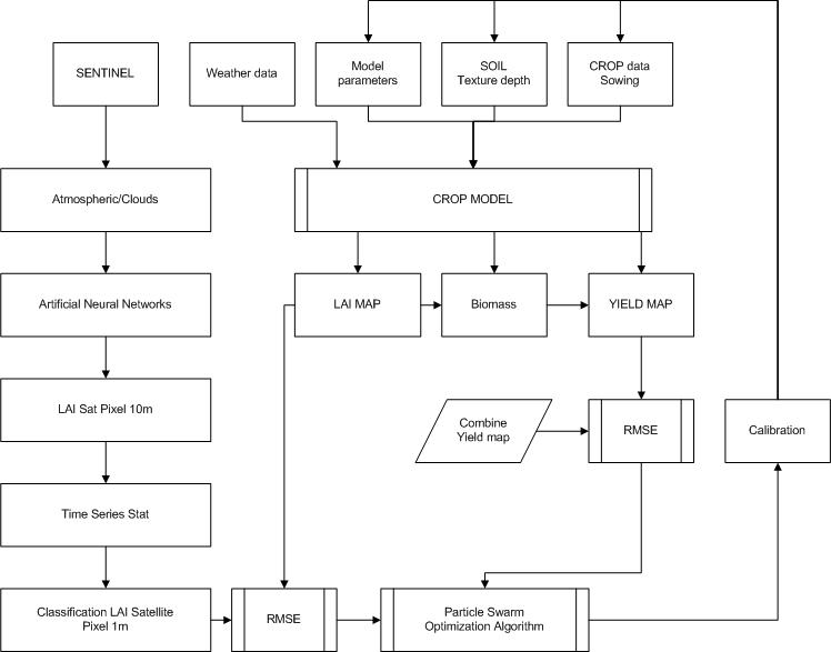
The diagram above describes the processes implemented, it breaks down into two main stages: a first which consists in using the satellite LAI in the model, we then minimize the RMSE (Root Mean Square Error) which is the difference between the LAI Sat and the LAI model by tuning soil parameters (soil depth, texture in defined ranges). The second step is to use a plot yield map to test the model or also calibrate its parameters in equations (Conversion from LAI to PAR (Photosynthetic Active Radiation, Harvest Index:conversion from biomass to yield). These two processes are completely independent, so we successively use the optimization algorithm twice to calibrate the model on two different objectives: LAI and yield.
The objective is to be able to run the models on a set of plots with yield maps to calibrate and then test the model according to conventional statistical processes. Once validated, the model can then be used without a yield card to predict the georeferenced yield early enough so that the farmer can intervene in the plot if necessary with a modulated irrigation dose, for example.
In this case, the model uses normal weather data from the plot location to make its calculations.
A test was carried out on a plot of Jean-Loup Chatard in the Allier department.
The video broadcast on its Youtube channel allows you to view the yield of this plot.
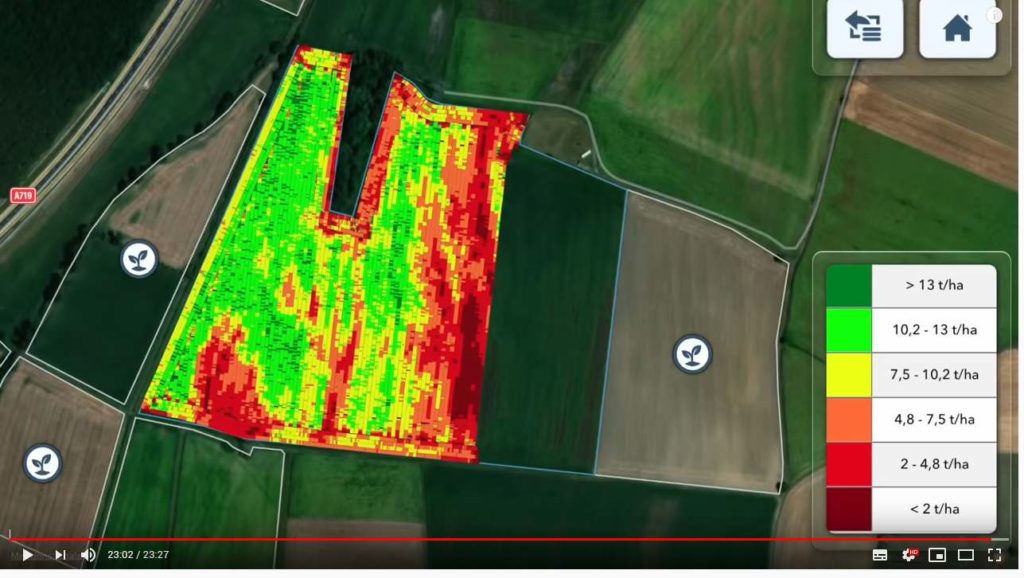
The processing of data from the machine is carried out with FieldView
On this plot the yield varies from 2t / ha to more than 13 T / ha, the origin of this variability is undoubtedly due to the heterogeneity of soils and available water for the plant.
The statistical analysis of the 7 images made it possible to calculate the following classification map by applying weights based on the date of the image, for the moment the weight is based on the number of days between the image and the date of maturity.
We then use this map to extract the LAIs time series in order to run the yield model as described in the diagram. These data are in reduced central variables in order to take into account the evolution of LAI during the season, exactly as we do in a neural network to be able to interpret data on different value scales. (Average equal to zero and standard deviation of one).
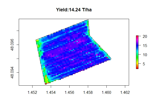
The average yield calculated on this plot is 8 T / ha, this must be fairly close to reality, a statistical examination of the yield map will allow us to go further in the analysis.
The next step will be to pass other yield maps on other geographical areas, the final objective of this work, is to be able to analyze all the plots of corn in a small region, and to determine the potential production early in the season with an index of probability of error that we would see decrease as we approach the harvest.