Most of the time, vegetation intra field variability is due to soil heterogeneity, in some cases, it can be due to different agricultural practices or tillage time. This is the case in that rapeseed field, sown on two different dates, as explained in a previous post.
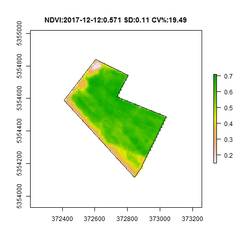
NDVI 12/12/2017 sowing date: 27/08/2017
The farmer objective is to minimize the field heterogeneity highlighted by the low NDVI values, not due to soil factor but to the sowing date (30/08/2017) causing low emergence rate after crust formation due to rainfall. (Silty soil)
During winter, one can expect that these areas will compensate the “wholes” in the field, probably, it is already visible in the NDVI sequence from the sowing date.
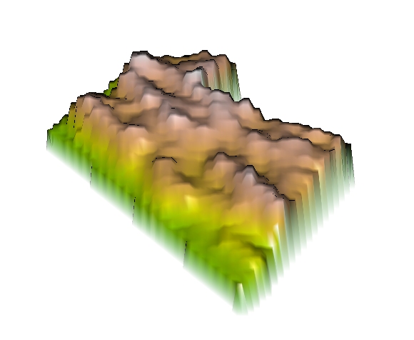
NDVI animation from sowing date

NDVI pixel density plot
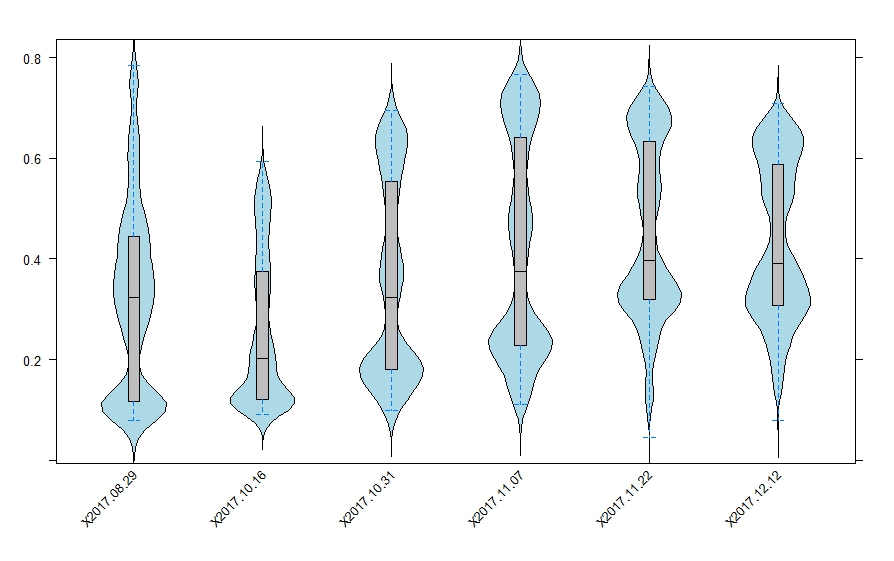
Bow and whisker plot
The above box plot is a godd visual indicator of NDVI level and dispersion along the six satellite images from the sowing date. The length of the whisker decreasing from 07/11/2017 indicate that standard deviation is decreasing (respectively 0.21,0.17,0.15 from 7/11/2017 to 12/12/2017)
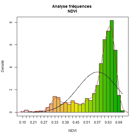
Frequential analysis 12/12/2017
The second sowing date is located on the first red curve mode. This lack of vegetation will be focused at the end of the winter, and possibly taken into account with the nitrogen modulation map by increasing amont level ih this area to compensate the vegetation lack.
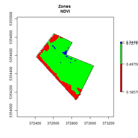
The above map is the simplest clustering map for a raster, according to the mean and the standard deviation (12/12/2017), pixels are classified function of the mean plus or minus the standard deviation, hence, red area highlight the lowest NDVI zones and the blue ones the highests.
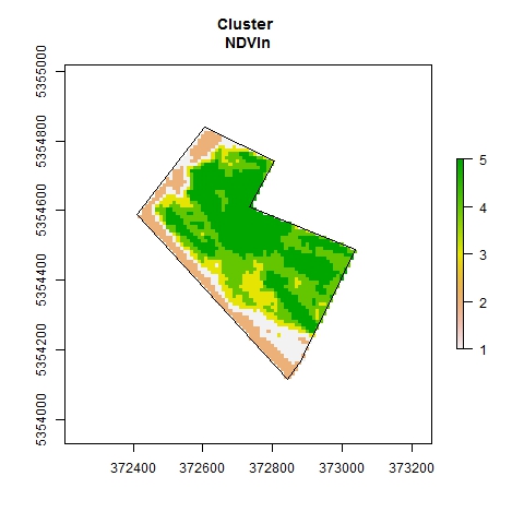
Cluster with 5 classes
One step ahead with a five classes clustering.
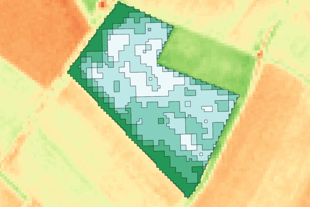
Nitrogen modulation map
And finally the system generate a nitrogen modulation map in a shape file format, ready to use in a precision sprayer. Here the nitrogen amount vary from 147 kgs/ha to 255 kgs/ha after leaf area, biomass and nitrogen uptake estimation.